Configuring real-time acquisition with scconfig
This chapter shows you how to import metadata for a set of stations into SeisComP. This is enough to begin processing in real time at your own installation.
The steps involved are:
- download metadata for the stations of interest,
- import them into your SC3 system, including bindings,
- view the stations and their traces in the SC3 GUIs.
Download station metadata
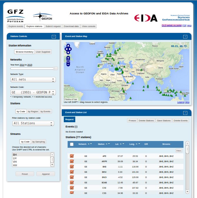
Download an inventory.xml or dataless SEED file from WebDC3 to request GEOFON stations (FDSN network code GE). (For a discussion of metadata formats, see Chapter Commonly used metadata formats with SC3.)
- Using the “Explore stations” tab, select the GE network, then ‘All Stations’
and BH (20 samples per second) streams
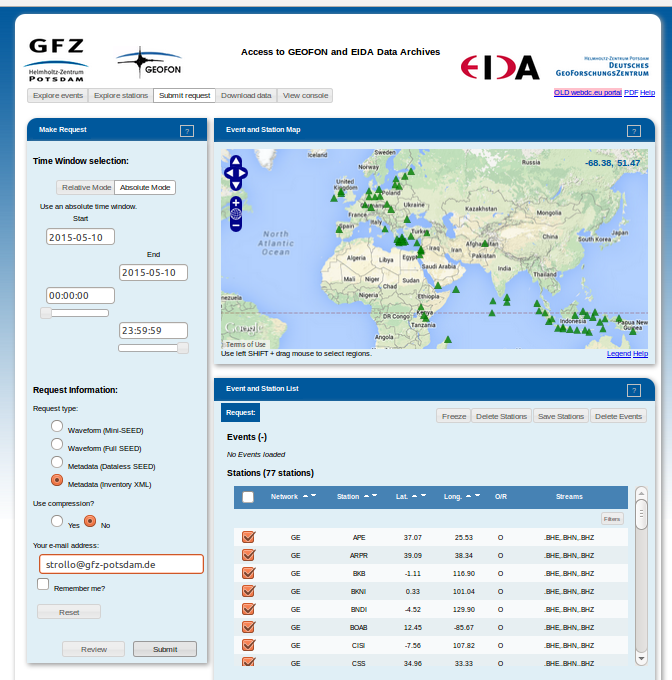
- Move to the “Submit request” tab and select Metadata (Inventory XML). Add your e-mail address and click on the “Submit” button.
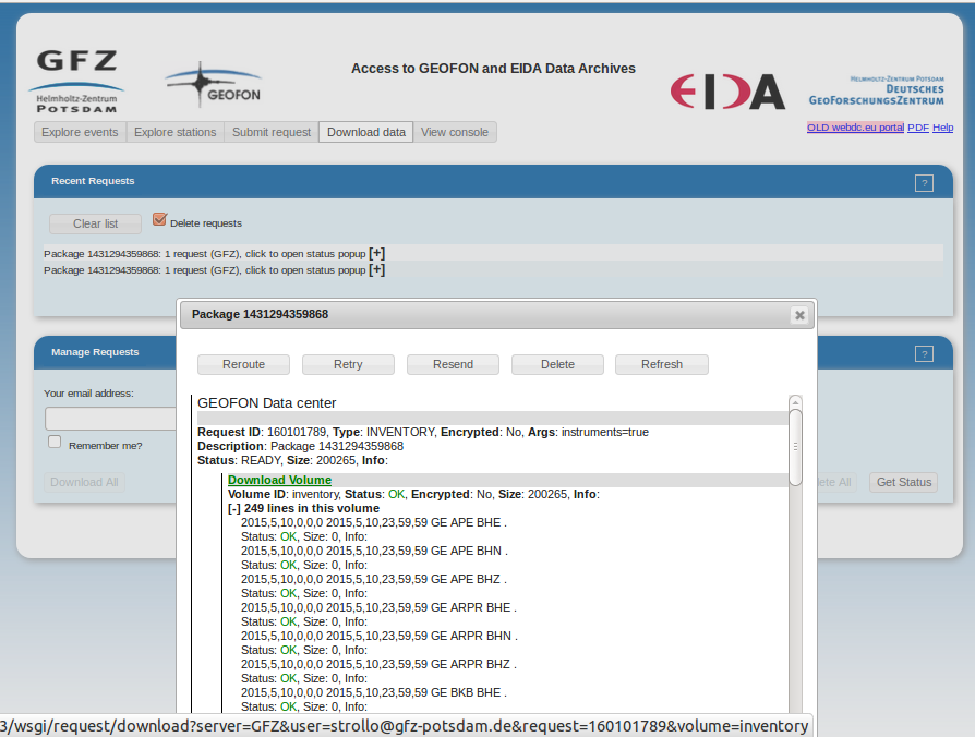
- Move to the “Download data” tab and click on [+] to see more information about the request. Click on “Download Volume” to save the data locally. Save the file as arclink_GE_BH.xml
Note
In case of a slow connection or large processing time, the dataset can be downloaded from http://geofon.gfz-potsdam.de/training/inventory/arclink_GE_BH.xml or http://geofon.gfz-potsdam.de/jakarta-2016/GE-inventory.xml .
Import the inventory
Start “scconfig” from a terminal. Select the “Inventory” icon on the left side bar.
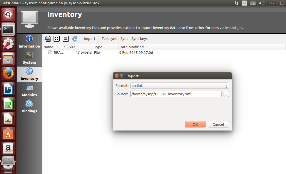
- Click on Import, select arclink format (for inventory.xml) or any format according to what you would like to import.
- Provide the path to your file in the “Source” field.
- Repeat the last two points you need to add additional metadata (remember to select the right format).
- Press the Sync keys button.
Configure Bindings
In SeisComP terminology, bindings are the connection between SC3 modules and individual stations. Within each module, stations can be differently configured; bindings determine how this happens. Full details are in the SeisComP documentation [1].
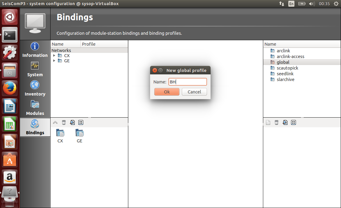
In scconfig, select the “Bindings” icon on the left side bar
- Create a global profile named “BH” by clicking with the right button on “global” in the top right panel. Double click on it and set BH as detectStream and empty location code as detecLocID information.
- If needed you may also create an “HH” global profile.
- Create a scautopick profile named “default” (no changes necessary).
- Create a seedlink profile named “geofon”. Double click on the profile. Add a chain source with the green plus button on the left (no other changes necessary).
- If you want to archive data, create a slarchive profile and name it “default”
(no other changes necessary).
- Drag and drop all profiles from the right side to the network icon on the left side (you may do that also at the station level).
- Press CTRL+S to save the configuration. This writes configuration files.
Update the configuration
The SeisComP database must be updated with the inventory and bindings, and the different SC3 modules require a restart to reload with the updated information.
Go to the system tab and press ESC (to deselect everything)
- Click on “Update configuration”, at the right of the window.
(Not “Update”, which just refreshes scconfig’s display of what is running!)
Press Start to start acquiring data from the already configured stations.
Start the GUIs
- Open scmv to see a map view of the configured stations.
- Open scrttv to see the incoming real-time streams.
If you see colored triangles and traces incoming it means that you have configured your system properly.
With this last step the basic setup is considered to be finished.
Footnotes
| [1] | Online at http://www.seiscomp3.org/doc/jakarta/current/apps/global.html |