Event simulation using synthetic waveforms
It is possible to generate mini-SEED data from a simulation of a seismic event. For a given set of hypothetical event parameters, this is quite quick, if pre-computed Greens functions are available.
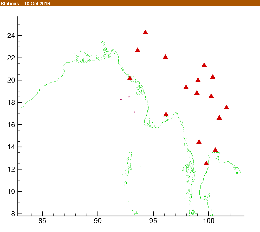
In this exercise, we use synthetic waveforms prepared by Dr Andrey Babyenko (GFZ Potsdam) corresponding to a large event in the Bay of Bengal, off the coast of Myanmar. Waveforms are prepared for 17 stations in Myanmar and Thailand.
The outline is:
- Given a sorted mseed data file, extract to local SDS archive.
- Locate as usual, either
- by automatic playback, or
- manually, by creating an artificial origin and loading waveforms in the picker.
In this introduction we only describe the second approach to location.
Extract sorted mini-SEED to local archive
Download the *.mseed files from the GEOFON training web site:
wget http://geofon.gfz-potsdam.de/training/resources/sc01.mseed
wget http://geofon.gfz-potsdam.de/training/resources/sc02.mseed
To avoid conflict with existing files in your standard SC3 archive (normally ~/seiscomp3/var/lib/archive) we will create a second SDS archive. We extract mini-SEED into this new archive:
cd ~/seiscomp3/var/lib
mkdir synth
cd synth
~/seiscomp3/bin/seiscomp exec scart -v -I sc01.mseed . >scart.out 2>&1
~/seiscomp3/bin/seiscomp exec scart -v -I sc02.mseed . >scart.out 2>&1
Don’t forget the dot (‘.’) at the end of the scart command! This causes scart to extract to the current working directory. Extraction should only take a few seconds. You will now have data in your archive directory e.g. ~/seiscomp3/var/lib/synth:
du -sh 2016
1.5M    2016/
ls 2016
IU  MM  RM  TM
Myanmar waveform playback reconfiguration
Ensure inventory contains the BH channels and their responses. (scinv ls > ~/scinv.out ; sed -n -e ‘/network MM/,/network /p’ ~/scinv.out | more should show channel BHE etc.)
If needed:
mv myanmar_MM_BH.xml ~/seiscomp3/etc/inventory
and use scconfig to sync inventory.
Adjust bindings:
- Create a global:MM profile. This lets you more easily switch between normal settings, using HH channels, and playback settings, using BH channels. Set detecStream = BH.
- Apply this profile to all MM stations. In scconfig, use CTRL+S to save.
- seiscomp update-config
To return to normal settings, open the global:MM profile, or edit ~/seiscomp3/etc/key/global/profile_MM. Change detecStream back to HH, and save. Do seiscomp update-config ; seiscomp restart scmaster.
Manual review
Start scolv, but with the ‘-I’ option telling it to use your new SDS archive as the record stream for obtaining waveforms:
scolv -I sdsarchive:///home/sysop/seiscomp3/var/lib/synth -u synscolv
Create an artifical origin:
- set origin time to 1 October 2016, 00:00:00
- set epicentre to 17N, 92E, depth 10 km.
Open the picker
- pick the first few stations.
- close the picker with the red button in the top right
Relocate. Note the location and residuals.
Pick additional stations, and return to the main scolv window.
Use the “Compute magnitudes” button to tell SeisComP to estimate a variety of magnitudes using this origin. Visit the Magnitudes tab to see the different magnitude estimates.
Click “Confirm” when you are happy with the solution.
The last step writes the event to the database. Next time you open scolv, you can go to the date of the event and refine your solution as necessary.
Automatic location
There are two sorts of automated playbacks, differing in whether the SC3 database is involved.
For an ‘’online’’ or ‘’waveform’’ playback, the database is connected as usual. Simulated objects (events, origins, picks) will all be inserted into the database. This can lead to confusion. However, this can be useful for watching the event unfold in the GUIs (scrttv, scmv, etc.)
The steps are:
Configure seedlink to work with a special file, a FIFO (first in, first out). The seedlink process reads from this, and another program, msrtsimul writes to it, reading from a sorted mini-SEED file. All processing continues as usual. The waveforms are stamped with the current time, instead of using the time at which they were recorded.
In scconfig, under Modules > seedlink: check “msrtsimul”. Save with CTRL+S. Under System > Update configuration.
Stop archiving (otherwise you will have copies of the old waveforms in your archive, but at the current time). Restart Seedlink.
seiscomp stop slarchive
seiscomp disable slarchive
seiscomp restart seedlink
If you are watching with scrttv, you will see waveforms stop. This is expected.
Feed in sorted mini-SEED:
msrtsimul file.mseedYou can try using the ‘–speed 1.5’ and ‘–jump 2’ options, to make the playback run a little faster, but this is not recommended. Some aspects of locating appear to get a little confused at speed > 1.
Watch the show in scrttv/scmv. Once the event is located, you can see it in scolv too.
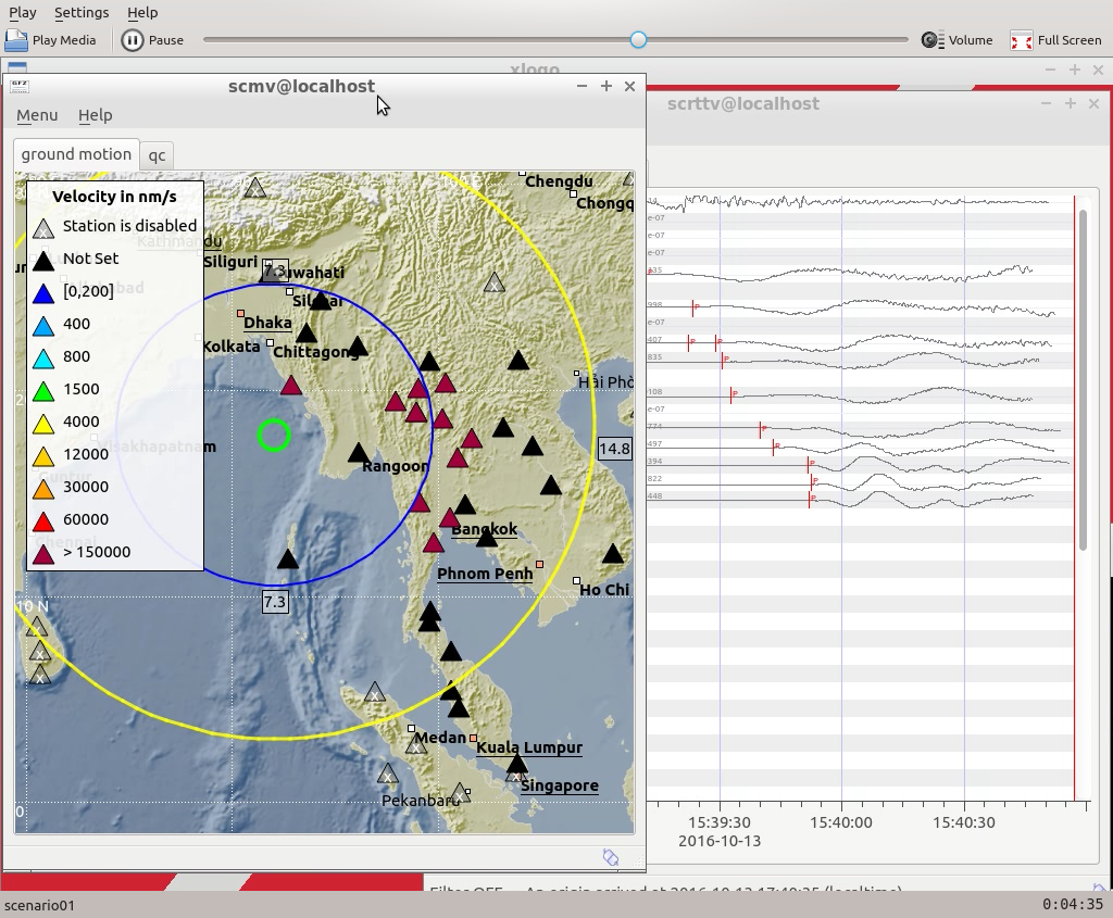
Screen shot from an online playback. On the left, scolv shows that a number of stations have detected a strong signal (dark red triangles). This has been automatically located, with the epicentre in the green circle. Yellow and blue circles show the expanding P and S wavefronts at this instant. There was no synthetic data available for stations shown by black triangles. On the right, scrttv shows waveforms in time. Red lines show automatic picks by scautopick.
For offline playback, see the Offline Data Playbacks chapter.
Production notes
We were given 400 seconds of simulated data. With 3 components, at 20 sps = 24000 samples per station, so this is just a few KB per station. After scart, see about 80-90 KB per station for the 17 stations in sc01.zip; files are for DOY 275 = 2016-10-01. Looks like 00:00:00; 400 seconds later is 00:06:40.